Introduction

The metropc framework provides machinery to implement a data pipeline configured and (re-)programmable at runtime by injected Python code. Data transformation is expressed as a collection of functions, so called views. A view takes input from one or more external data sources and may return a result, which in turn serves as input to other views. The execution of views occurs on an event boundary, with each event forming a graph of executed views and their corresponding results.

Typical applications are online analysis from slicing data to a custom region of interest over performing simple statistical analyses to extensive pipelines processing raw data with complex algorithms in realtime. As the underlying analysis code can be changed quickly at runtime, it allows for fast iterations and explicit implementations to solve a given problem in the very same moment. In general, any operation that can be expressed with Python may be performed. This also includes calling native code or bindings to larger frameworks, e.g. OpenCL or CUDA. The graph of views shown above may be implemented like this:

import numpy as np
import xarray as xr
from my_analysis_library import correct_background

# Do background correction for input A, add custom axes to A and B,
# calculate the interpolated quotient and average it.

@View.Compute
def preprocess_A(data: 'input_A'):
    # Correct background for input A.
    return correct_background(data)

@View.Vector
def process_A(data: 'preprocess_A'):
    # Add calibration axis specific for A.
    return xr.DataArray(data, dims=['position'],
                        coords={'position': np.linspace(0, 1, len(data)))

@View.Vector
def process_B(data: 'preprocess_B'):
    # Add calibration axis specific for B.
    return xr.DataArray(data, dims=['position'],
                        coords={'position': np.linspace(0, 1, len(data)))

@View.Vector
def combine_AB(data_A: 'process_A', data_B: 'process_B'):
    # Calculate interpolated quotient.
    common_axis = np.linspace(0, 1, min(len(data_A), len(data_B)))
    return data_A.interp(position=common_axis) / data_B.interp(position=common_axis)

@View.Vector_MovingAverage(N=20)
def average_AB(AB: 'combine_AB'):
    return AB

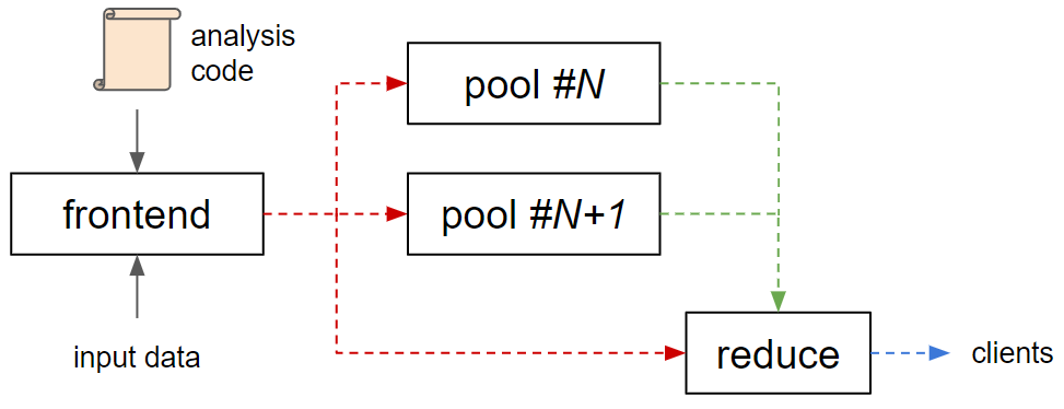
The pipeline consists of several stages each with different semantics. As a framework, metropc needs to be embedded in an application called its frontend. Its purpose is to control all pipeline stages and feed external data into it for processing. The following pool stage serves as the primary location for all computations limited to the data contained in a singular event. Any number of pool instances may run concurrently in different processes or even nodes for load balancing and as such, there is no guarantee of a common scope across any two events. This is different in the subsequent reduce stage, of which exactly one instance is present in any pipeline. It allows to perform reductions across several events such as averages or other statistics. As each event passes synchronously through this stage, the time available for computations per event is limited by the desired output rate.

All these components may run on a single machine in different threads and processes or be spread across multiple nodes, both the individual stages as a whole as well as individual instances, e.g. in the pool stage. All internal and external communication is handled by ZeroMQ, which can scale from zero-copy transfer between threads (inproc://) to processes (ipc://) and nodes (tcp://). First, there is the control connection between the frontend (ROUTER) and all stage instances (REPLY) for event input and pipeline management. The reduce connection forwards data from the pool stage instances (PUSH) to the reduce stage (PULL). Finally, the output connection in the reduce stage (PUB) sends data to any connected client (SUB).

These documentation describes the core framework itself and is largely frontend-agnostic. At European XFEL, you most likely want to use the MetroProcessor Karabo device for online data, or the extra-metropc-run installed with metropc command for offline data.