In this project, the participants will learn to model multiphoton multiple ionization dynamics of atoms exposed to intense x-ray radiation. The participants will evaluate crucial quantities and pulse-parameter dependencies that are relevant for high-intensity AMO experiments at XFEL sources. Such theoretical modelling is often applied at experiments where multiple x-ray ionization occurs, for example in Refs. [6, 4, 2, 1].
You need to install the XATOM software, which is part of XRAYPAC. Please find instructions to download and install XRAYPAC on the website https://desy.de/~xraypac. The content of this exercise and all required files may be obtained from https://gitlab.desy.de/CDT/tutorialratesolving.git.
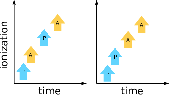
The intense x-ray light in an XFEL pulse can ionize the sample many times. When molecules or atoms are exposed to such pulses, the overall dynamics can be modelled via sequential steps that describe a series of photoionization, Auger decay, and fluorescence processes. Such sequences (without fluorescence) are sketched in Fig. 1.
The involved multiphoton multiple ionization dynamics can be modeled to a good approximation via rate equations of the type
| (1) |
where pi(t) is the time-dependent population of an electronic configuration i and γj→i(t) is a transition rate for a process between configuration j and i. In this exercise, we consider the following types of processes:
Motivation: Analytically solve the rate equation, derive dependecies for the competition of photoionization and Auger-Meitner decay.
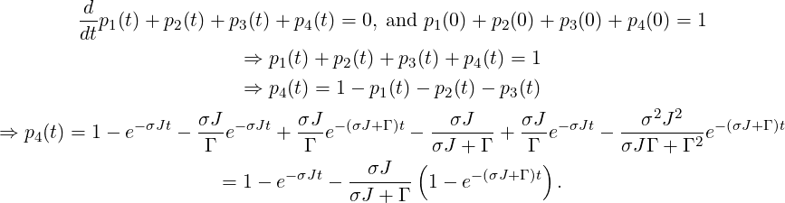
Given is the following set of rate equations:
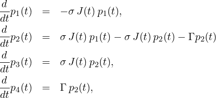
with the boundary conditions p1(0) = 1, p2(0) = 0, p3(0) = 0, p4(0) = 0, and a temporal step-function for the fluence,
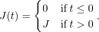 |
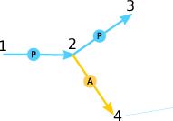
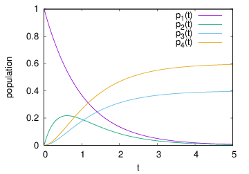
This set of rate equations models the competition between Auger-Meitner decay and photoionization illustrated in Fig. 2: The ionization dynamics start with photoionization from electronic configuration 1 into configuration 2. Configuration 2 can either further be photoionized into configuration 4 (a PP sequence) or undergo Auger-Meitner decay into configuration 3 (a PA sequence). The possible pathways are also illustrated by the graph on the right hand side of the rate equation.
Give the analytical solution and plot them for varying parameters σJ and Γ. Help: For
p2(t), you may consider the ansatz p2(t) = λ(t)exp(−(σJ + Γ)t). Alternatively, you may
consider using the Laplace transformation. What is the probability to observe PP vs. PA
process?
_______________________________________________________________________________________
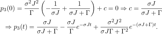
p1(t) can be solved by separation of variables and integration. The solution is (t ≥ 0)
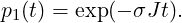 |
This yields for p2(t), t ≥ 0
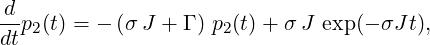 |
which is an inhomogeneous first-order differential equation. It can be solved employing the Ansatz p2(t) = λ(t)exp(−βt), with β = σJ + Γ (homogeneous solution + variation of constant). This yields
![− βt d −βt −βt −σJt
e dtλ(t) − βe λ(t) = − βλ(t)e + σ J e ,
-d (β−σJ)t --σJ--- (β−σJ)t
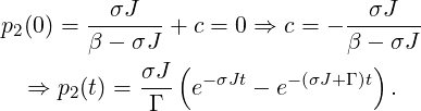
dtλ(t) = σJ e ⇒ λ (t) = β − σJ e + c
[ ]
⇒ p2(t) = --σJ---e(β−σJ)t + c e−βt.
β − σJ](exerciseSheet_solution5x.png)
The solution for p3(t) is obtained as follows:

| (2) |
yields
The solution for p4(t) with t ≥ 0 is obtained as follows:
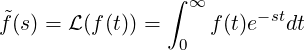
Alternatively, the solution can be obtained via Laplace transformation. Consider the Laplace transformation
| (3) |
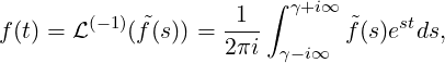
and the back-transformation
| (4) |
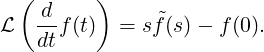
where the parameter γ is larger than the real part of any singularity of f(s). It holds that
| (5) |
Using the Laplace transformation, the coupled rate equations for t ≥ 0 can be written as
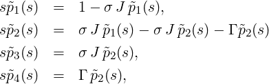
This can be directly solved and back-transformed:
| p1(s) | =  | ||
| ⇒ p1(t) | = exp(−σJt) | ||
| p2(s) | =  p1(s) = p1(s) =   = =   | ||
| ⇒ p2(t) | =   | ||
| p3(s) | =  p2(s) = p2(s) =    | ||
=   | |||
| ⇒ p3(t) | =   | ||
| p4(s) | =  p2(s) = p2(s) =   | ||
= σ J | |||
| ⇒ p4(t) | = σ J | ||
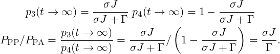
In this example, the probability to observe PA or PP process is directly given by the populations p3 and p4 at t →∞.
The transition rates for the electronic processes can be calculated using ab-initio methods. Here a short overview of the basic equations is given. See Ref. [3] for further details.
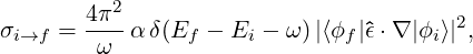
The photoionization cross section (in dipole approximation and assuming effectively independent electrons) is given by
| (6) |
where ω is the photon energy, Ef and Ei are the effective one-particle energies, ϕf and ϕi are the corresponding one-electron wavefunctions, 𝜖 is the polarization vector of the light field, and ∇ = (∂x,∂y,∂z)T .
Employing similar approximations on the electronic wave function, the Auger-Meitner decay rate from an initial electronic state with a core vacancy in orbital ϕc(r) (otherwise closed shell) and a final electronic state with two vacancies in ϕv1(r) and ϕv2(r) and an Auger-Meitner electron with continuum wave function ϕk(r) is given by
| (7) |
where
| (8) |
and Ev1, Ev2, Ec, and Ek are the corresponding one-particle energies.
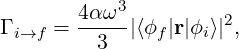
The fluorescence rate is given by
| (9) |
where ω = Ei − Ef is the emitted fluorescence photon energy, and ⟨ϕf|r|ϕi⟩ is the transition dipole moment between the the initially occupied orbital ϕi and the initially vacant orbital ϕf.
The calculation of the respective transition rates can be a challenge on its own. They can be obtained
by available electronic structure programs. In this course, we employ the atomic electronic structure
program XATOM [5]. XATOM calculates transition rates employing the Hartree-Fock-Slates electronic
structure model. All the obtained transition rates are average over the spin-angular terms for a given
atomic configuration. For example, the cross section for core-shell ionization of a neutral, ground state
carbon atom (configuration 1s22s22p2) is a weighted average over all the involved atomic terms 1S, 3P,
1D.
Motivation: Learn how to use the electronic structure tool XATOM to calculate rates and cross-sections.
Make yourself familiar with the XATOM tool. You can calculate the electronic structure of a neon atom by typing
To calculate a specific electronic configuration of neon use
To calculate a photoionization cross section for a given photon energy use
Decay rates (for Auger-Meitner and fluorescence) can be calculated via
Moreover, you can get a short overview of command-line options with
Further usage is described in the pdf document “xatom_manual.pdf” in the project folder.
Calculate the photoionization cross section for neutral neon and ionized neon as a function of photon energy from 400 eV to 1000 eV. Plot the results (you may use any plot program you like).
Calculate the lifetime of core-ionized (configuration 1s12s22p6), doubly core-coreionized (configuration
1s02s22p6) neon, and core and valence-ionized neon (e.g., configuration 1s12s22p0). Compare the
numbers. Can you explain why one is considerably larger?
_______________________________________________________________________________________
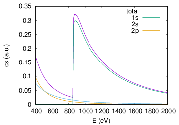
The photoionization cross section shows an edge at ≃ 860eV because at this energy ionization of the 1s shell becomes available.
The lifetime of the neon 1s−1 configuration is 2.5 fs, and the lifetime of the neon 1s−2 configuration
is 0.8 fs, the lifetime of the configuration 1s12s22p0 is 13.4 fs. The double-core hole decays much faster
because each core hole can be refilled via Auger-Meitner processes. In addition, the double-core-hole
lifetime is even shorter than half the single-core-hole lifetime, because of valence orbitals are more tight
around the core and thus interaction integrals become larger. Holes in the valence increase the
core-hole lifetime because electrons for Auger-Meitner and fluorescence decay channels are missing.
_______________________________________________________________________________________
The python notebook rateSolver_Solution.ipynb(html) contains a code for numerically solving rate
equations. To solve the rate equations with this code, a table of rates and cross sections needs to be
prepared that is fed into the numerical solver. The table for the previous 4-configuration example with
parameters σ = 1, Γ = 3∕2, and J = 1 is already provided.
For neon, a table of rates and cross sections for a photon energy of 2 keV is also already provided. It
has been generated with the python notebook tableGeneration.ipynb (html). Feel free to inspect it.
You may also want to modify it to address other elements or further photon energies. In order to use it,
you have to set XATOMPATH tp the path of your XATOM binary. Please consider that for larger atoms
the number of electronic configurations explodes dramatically. For such atoms, solving the
rate equation with tabulated rates thus becomes infeasible and other approaches have to be
taken.
Motivation: Learn how to solve the rate equations for a realistic scenario using numerical solver.
Modify the notebook to verify your previous analytical solution with the numerical one. Add the
required code into blank cells in the notebook.
In the python notebook rateSolver_Solution.ipynb(html) the rate equations are solved for the provided table of rates and cross sections for neon. Make yourself familiar with the code. The variable nPhotonsperSqmuM specifies the number of photons per μm2, the variable fwhmPulse specifies the full width at half maximum of the temporal pulse profile. Because of the many configurations involved, it is tedious to inspect the solution for every single configuration. Instead, the average charge is shown and the population of charge states (summing up the populations for configurations with the same charge state). The probability for PP vs. PA sequence is calculated as well. Try to change the parameters fluence and pulse duration and inspect how the results change.
Modify the notebook such that you generate plots of the average charge as a function of fluence and as a function of pulse duration. Add your code in the blank cells of the notebook. Plot the average final charge as a function of fluence for a given pulse duration. Plot the average final charge as a function of pulse duration for a given fluence. Plot the ratio of PP processes vs. PA processes as a function of fluence and pulse duration. Explain the observation.
Consider the notebook tableGeneration.ipynb (html). Can you do your analysis for another
photon energy, e.g., 1 keV?
[1] T. Jahnke, R. Guillemin, L. Inhester, S.-K. Son, G. Kastirke, M. Ilchen, J. Rist, D. Trabert, N. Melzer, N. Anders, T. Mazza, R. Boll, A. De Fanis, V. Music, Th. Weber, M. Weller, S. Eckart, K. Fehre, S. Grundmann, A. Hartung, M. Hofmann, C. Janke, M. Kircher, G. Nalin, A. Pier, J. Siebert, N. Strenger, I. Vela-Perez, T. M. Baumann, P. Grychtol, J. Montano, Y. Ovcharenko, N. Rennhack, D. E. Rivas, R. Wagner, P. Ziolkowski, P. Schmidt, T. Marchenko, O. Travnikova, L. Journel, I. Ismail, E. Kukk, J. Niskanen, F. Trinter, C. Vozzi, M. Devetta, S. Stagira, M. Gisselbrecht, A. L. Jäger, X. Li, Y. Malakar, M. Martins, R. Feifel, L. Ph. H. Schmidt, A. Czasch, G. Sansone, D. Rolles, A. Rudenko, R. Moshammer, R. Dörner, M. Meyer, T. Pfeifer, M. S. Schöffler, R. Santra, M. Simon, and M. N. Piancastelli. Inner-Shell-Ionization-Induced Femtosecond Structural Dynamics of Water Molecules Imaged at an X-Ray Free-Electron Laser. Phys. Rev. X, 11(4):041044, December 2021.
[2] A. Rudenko, L. Inhester, K. Hanasaki, X. Li, S. J. Robatjazi, B. Erk, R. Boll, K. Toyota, Y. Hao, O. Vendrell, C. Bomme, E. Savelyev, B. Rudek, L. Foucar, S. H. Southworth, C. S. Lehmann, B. Kraessig, T. Marchenko, M. Simon, K. Ueda, K. R. Ferguson, M. Bucher, T. Gorkhover, S. Carron, R. Alonso-Mori, J. E. Koglin, J. Correa, G. J. Williams, S. Boutet, L. Young, C. Bostedt, S.-K. Son, R. Santra, and D. Rolles. Femtosecond Response of Polyatomic Molecules to Ultra-intense Hard X-rays. Nature, 546(7656):129–132, May 2017.
[3] Robin Santra. Concepts in x-ray physics. J. Phys. B: At. Mol. Opt. Phys., 42(2):023001, December 2008.
[4] Sang-Kil Son and Robin Santra. Monte Carlo calculation of ion, electron, and photon spectra of xenon atoms in x-ray free-electron laser pulses. Phys. Rev. A, 85(6):063415, June 2012.
[5] Sang-Kil Son, Linda Young, and Robin Santra. Impact of hollow-atom formation on coherent x-ray scattering at high intensity. Phys. Rev. A, 83(3):033402, March 2011.
[6] L. Young, E. P. Kanter, B. Kraessig, Y. Li, A. M. March, S. T. Pratt, R. Santra, S. H. Southworth, N. Rohringer, L. F. DiMauro, G. Doumy, C. A. Roedig, N. Berrah, L. Fang, M. Hoener, P. H. Bucksbaum, J. P. Cryan, S. Ghimire, J. M. Glownia, D. A. Reis, J. D. Bozek, C. Bostedt, and M. Messerschmidt. Femtosecond electronic response of atoms to ultra-intense X-rays. Nature, 466(7302):56–61, July 2010.