Example (GAMESSUS): Excited H2O+ in external electric field (BO+FSSH)
This example describes the interaction of a water molecule ion in a time-dependent electric field. See directory:
Examples/xpyder/h2o+_field/
Preparation
Set your environment variable CDTK_GAMESSUS to the path of the gamessus directory. For example:
export CDTK_GAMESSUS=$HOME/gamess/
Instead of ‘$HOME/gamess/’ insert the actual path of your gamess installation.
Depending on your gamess installation, output is written to the scratch file folder. This is configured in the
rungmsscript in your gamess installation. Edit the scriptrungmsaccordingly so that the output is written in the current working directory. You may want to comment out the linesset SCR=~/gamess/restartand#set USERSCR=~/gamess/restart, instead, set the SCR and USERSCR environment variables to.. For example:export SCR=. export USERSCR=.
Note that the local directory in which the simulation is run should be a rapidly accessible disk (i.e., a local folder or ramdisk) - otherwise there will be huge performance losses.
Run the BO dynamics
To run the example, execute:
xpyder -i input_bo_es -d bo_es
Details of the Inputfile
The file input_bo_es is the input file used for the calculation:
$SYSTEM
    qchemistry  = gamess
    xunit       = an
$END

$gamess
    memddi = 2
    mwords = 2
    gbasis = CCD
    icharg = 1
    mult = 2
    ncore = 1
    nact = 4
    nels = 7
    wstate = 1.0,1.0
    nstate = 4
    sz = 0.5
    mxxpan = 100
    fullnr = .false.
$end

$trajectory
    dt = 0.5   fs
    tf = 40.0   fs
$end

$quantum
    type    = bo
    istate  = 1
    nstates = 2
$end

$cartPOS
 O    0.0   0.0        0.0
 H    0.0   0.757215   0.5865358
 H    0.0  -0.7572157  0.5865358
$end

$cartVEL
 O  0.0  0.0  0.0
 H  0.0  0.0  0.0
 H  0.0  0.0  0.0
$end


$efield
    envelope =  gaussian
    omega =     4000.0   cm-1
    fwhm =      10      fs
    phase =     0.5
    center =    15 fs
    amplitude = 0.104   au
    #amplitude = 0.0   au
    polarization = 0.0  0.0  1.0
$end
The section
$SYSTEMqchemistry = gamessspecifies the quantum chemistry tool. (One can also give “molcas”, but remember that field induced dynamics cannot be done using MOLCAS with the current version of CDTK).xunit = anspecifies the unit in the coordinates of the atom is specified. “an” refers to Angstrom and one can give “au” for atomic units.
$gamessthis gives the input detials such as the basis used, active space etc., for the electronic structure calculation.
$trajectory- “dt” specifies the time step used for the calculation (in fs). - “tf” specifies the final time ie., the time till the calculation will last (in fs).quantumtype = bospecifies Born-Oppenheimer dynamics. That means we stay at a fixedistateandnstategives the initial state at which the trajectory present and the nomber of states respectively.
cartPOSandcartVEL. This gives the intial position and velicity of the atoms.$efieldspecifies an electric field.envelopegives the shape of the envelope. Currently, the only possible value is “gaussian”omegasecifies the central frequencyamplitude,fwhm,phase, andcenterspecify the temporal width as the full width at half maximum , the phase
  (in rad), and the temporal center
  ,
such that the temporal envelope of the electric field is given by
,
such that the temporal envelope of the electric field is given by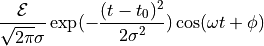
with
 and
and  is the amplitude of the electric field.
polarizationspecifies the polarization (x, y, z, value)
Output data
The folder bo_es contains all the output files.
R.loggives the position of the atoms: The first column is time; the following columns coordinates (x,y,z) for each atom. All columns are in atomic units.V.loggives the velocity of the atoms: The first column is time; the following columns velocities (x,y,z) for each atom. All columns are in atomic units.E.logcontains 4 columns (all in atomic units): The first column gives the time, the second column gives the kinetic energy, the third column gives the potential energy, and the fourth column the total energy (sum of kinetic and potenital energy) of the simulation trajectory.field.logcontains 3 columns: First column time (in atomic units), second column the amplitude of the electric field (in atomic units) and the third column gives the temporal envelope of the electric field pulse (in atomic units).
You can convert the trajectory information into .vtf format or .xyz format by executing either an_traj2vtf or cdtk2xyz.
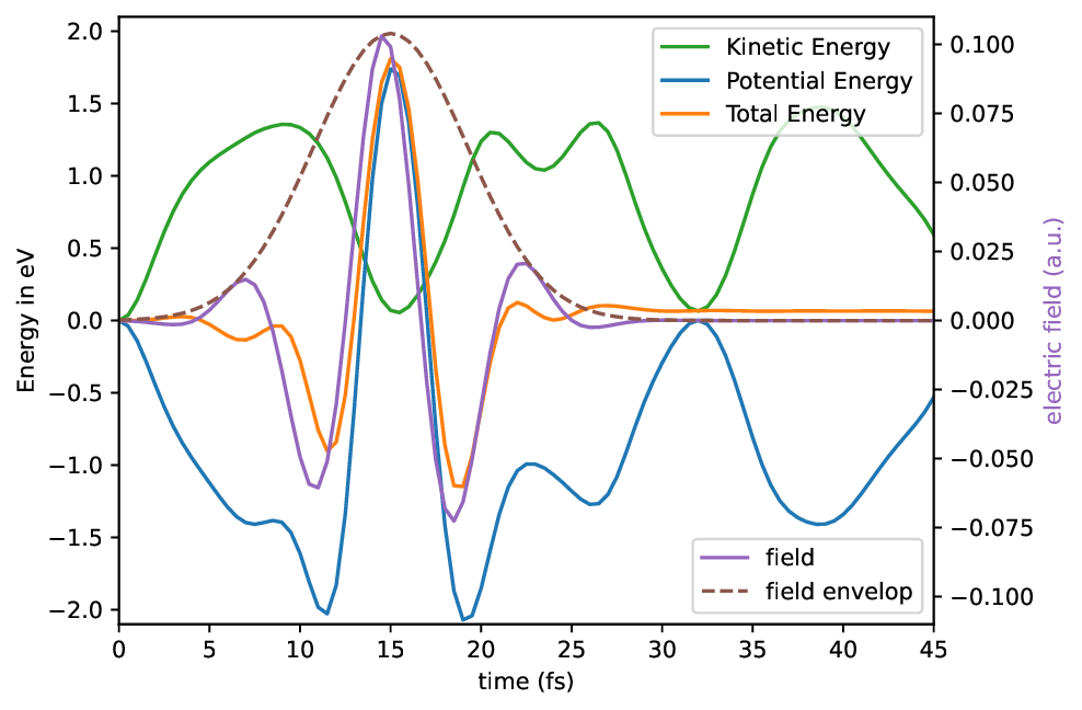
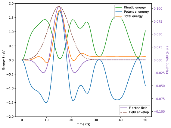
Electric field, total molecular energy, potential and kinetic energy as a function of time.
Animation of water molecule cation exposed to time dependent electric field.
As one can see, in the ionized and excited state the water molecule strongly vibrates. The external field along the z direction pushes and pulls the water molecule and thus modifies the vibration. As a consequence the total energy of the molecule after the pulse is somewhat altered. It turns out, the total energy can be increased by the pulse, when the electric field pushes the hydrogen atoms along the vibration, or it can be decreased by the pulse, when the electric field pushes the hydrogen atoms against the vibration:
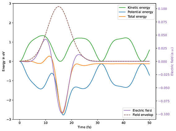
Electric field, total molecular energy, potential and kinetic energy as a function of time.
Here a frequency of  has been used and a phase of
  .
.
Electric field, total molecular energy, potential and kinetic energy as a function of time.
Here a frequency of has been used and a phase of  .
.
Running the dynamics using fewest switches surface hopping
A variant for this example employing fewest switches surface hopping can be found here:
Examples/xpyder/h2o+_field/input_fssh
Compared to the earlier example, the input file is changed in the section:
$gamess
   memddi = 2
   mwords = 2
   gbasis = CCD
   icharg = 1
   mult = 2
   ncore = 1
   nact = 4
   nels = 7
   wstate = 1.0,1.0,1.0,1.0
   nstate = 4
   sz = 0.5
   mxxpan = 100
   fullnr = .false.
$end
altering the GAMESS calculation parameters and in the section:
$quantum
   type    = fssh
   istate  = 1
   nstates = 4
$end
switching on the surface hopping. Moreover, the polarization of the electric field is changed and now in the x-axis direction:
$efield
   envelope =  gaussian
   omega =     4000.0   cm-1
   fwhm =      10      fs
   phase =     0.5
   center =    15 fs
   amplitude = 0.104   au
   polarization = 1.0  0.0  0.0
$end
Run the FSSH dynamics
To run the example, execute:
xpyder -i input_fssh -d fssh
For comparison you may also run the example without any external field (amplitude set to zero):
xpyder -i input_fssh_nofield -d fssh_nofield
Output data
The folders fssh fssh_nofield contain all the output files. In addition to the earlier example, these are
P.logcontains the electronic populations as a function of time.C.logcontains the electronic state coefficients as a function of time.S.logcontains the active state as a function of timeV_ad.logcontains the adiabatic potential energies as a function of time.
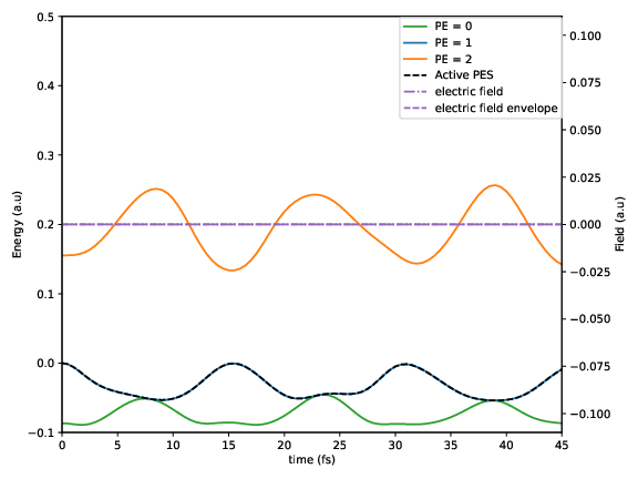
Without electric field |
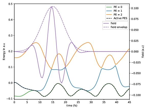
With electric field |
|---|---|
|
|
|

|
The figures show how the electric field enables non-adiabatic transitions: In the trajectory with electric field, the active potential energy surface changes at time t=7fs.
Further example
Further examples with CO2 can be found here:
Examples/xpyder/co2_field/