Example (XMOLECULE): Dynamics of H₂O⁺ with a classical electron

In this example, the dynamics of an ionized water molecule and an electron in its vicinity is described. The example investigates the interaction of the molecule ion and a photoelectron during a photoionization process.

See:

Examples/xpyder/H2O+_and_el/

Preparation

Make sure you have installed xmolecule in your local python environment. See Installation instructions.

Running

To execute the example run:

xpyder -i input_electron_fssh -d electron_fssh

Details of the Inputfile

The input_electron_fssh is the input file used for the calculation:

$SYSTEM
  qchemistry = xmolecule
  xunit = bohr
$END

$xmolecule
  MOM=yes
  gto=6-31G
  HF=yes
  gs_occ=yes
  occ=22221
  charge=1
  R_softcore=0.32
$end

$trajectory
  dt = 0.001   fs
  tf = 1.0   fs
$end

$quantum
  type = fssh
  nstates = 4
  istate  = 3
  rescaling = nac
$end

$mmregion
  dt = 0.001  fs
$end


$cartPOS
  O  -0.000000    -0.000000     0.116743
  H  -0.000000    -1.498103     1.205793
  H  -0.000000     1.498103     1.205793
$end

$cartVEL
  O     0.000000     0.000000     0.000000
  H     0.000000     0.000000     0.000000
  H     0.000000     0.000000     0.000000
$end

$cartPOS_MM
  e    0.000000     0.600000     0.600000
$end

$cartVEL_MM
  e    0.000000     0.100000     0.600000
$end

1. $SYSTEM

   • qchemistry = xmolecule specifies the quantum chemistry tool.

2. $xmolecule gives input details for the electronic structure calculation

3. $trajectory

   • dt is for the time step used for the calculation (in fs).

   • tf is the final time ie., the time till the calculation will last (in fs)

4. $quantum

   • type = fssh specifies the type of surface hopping. fssh denotes Tully’s Fewest Switches Surface hoping.

   • istate and nstate gives the initial state at which the trajectory starts and the number of states that are used, respectively.

   • rescaling = nac specifies the type of rescaling done.

4. $mm_region indicates that there is a classical particle in the simulation

5. $cartPos / $cartPos_MM / $cartVEL / $cartVEL_MM

   • these section specify the initial position and velocities of the atoms and the electron

Output data

The folder electron_fssh contains all the output files.

1. P.log gives the population of the states by solving the time dependent Schroedinger equation.

2. C.log gives the co-efficients of the states.

3. V_ad.log gives the adiabatic potential energies for all the states.

4. R.log gives the position of the atoms and the electron.

5. V.log gives the velocity of the atoms.

6. S.log gives the state at which the trajectory is at every time step.

7. NAC.log gives the coupling terms i.e., the off diagonal terms of the Hamiltonian.

8. E.log gives the potential energy, kinetic energy and totol energy of the trajectory.

9. Switch.log gives the details of the hopping, its probability, the random number used and also more details about the hopping.

10. partial.log shows partial charges of each atom (Mulliken charges).

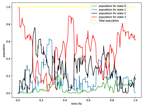
Electronic state populations as a function of time.

The figure shows the electronic state populations as a function of time computed for a single FSSH trajectory. As one can see, the flying away electron induces strong couplings between the states that leads to strong changes in the state populations.